Klein bottle
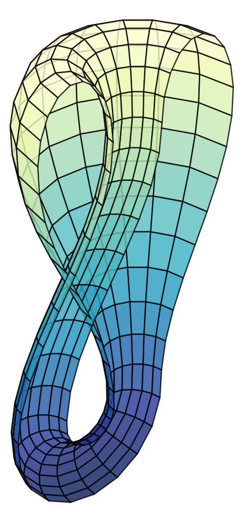
In mathematics, the Klein bottle /ˈklaɪn/ is an example of a non-orientable surface; it is a two-dimensional manifold against which a system for determining a normal vector cannot be consistently defined. Informally, it is a one-sided surface which, if traveled upon, could be followed back to the point of origin while flipping the traveler upside down. Other related non-orientable objects include the Möbius strip and the real projective plane. Whereas a Möbius strip is a surface with boundary, a Klein bottle has no boundary (for comparison, a sphere is an orientable surface with no boundary).
The Klein bottle was first described in 1882 by the German mathematician Felix Klein. It may have been originally named the Kleinsche Fläche (“Klein surface”) and then misinterpreted as Kleinsche Flasche (“Klein bottle”), which ultimately may have led to the adoption of this term in the German language as well.
The following square is a fundamental polygon of the Klein bottle. The idea is to ‘glue’ together the corresponding coloured edges so that the arrows match, as in the diagrams below. Note that this is an “abstract” gluing in the sense that trying to realize this in three dimensions results in a self-intersecting Klein bottle.
Construction
Source: Wikipedia
Kinds of Expressions
Among basic expressions are literals, for example, decimal (real), enumeration, string, and access value literals:
2.5e+3
False
"и"
null
Involving many of those one can write aggregates (a primary),
(X => 0.0,
 Y => 1.0,
 Z => 0.0)
Arbitrarily complex sub-components are possible, too, creating an aggregate from component expressions,
(Height => 1.89 * Meter,
 Age    => Guess (Picture => Images.Load (Suspects, "P2012-Aug.PNG"),
 Tiles   => Grid'(1 .. 3 => Scan, 4 => Skip)),
 Name   => new Nickname'("Herbert"))
Age is associated with the value of a nested function call. The actual parameter for Tiles has type name Grid qualify the array aggregate following it; the component Name is associated with an allocator.
The well known ‘mathematical’ expressions have closely corresponding simple expressions in Ada syntax, for example 2.0πr, or the relation
Area = π*r**2Other expressions test for membership in a range, or in a type:
X in 1 .. 10 | 12
Shape in Polygon'ClassHexagonal Torus
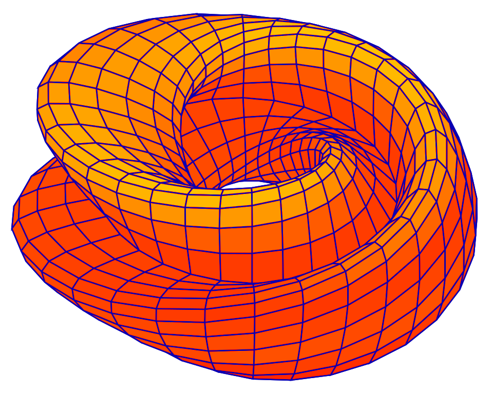
In geometry, a torus (plural tori) is a surface of revolution generated by revolving a circle in three-dimensional space about an axis coplanar with the circle. If the axis of revolution does not touch the circle, the surface has a ring shape and is called a torus of revolution.
Real-world examples of toroidal objects include inner tubes, swim rings, and the surface of a ring doughnut or bagel.
A torus should not be confused with a solid torus, which is formed by rotating a disk, rather than a circle, around an axis. A solid torus is a torus plus the volume inside the torus. Real-world approximations include doughnuts, vadai or vada, many lifebuoys, and O-rings.
In topology, a ring torus is homeomorphic to the Cartesian product of two circles: S1 × S1, and the latter is taken to be the definition in that context. It is a compact 2-manifold of genus 1. The ring torus is one way to embed this space into three-dimensional Euclidean space, but another way to do this is the Cartesian product of the embedding of S1 in the plane. This produces a geometric object called the Clifford torus, a surface in 4-space.
In the field of topology, a torus is any topological space that is topologically equivalent to a torus.
Source: Wikipedia
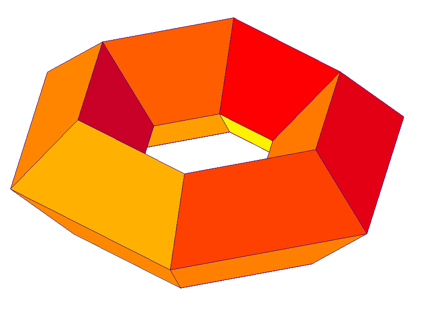
Heesch’s polygon
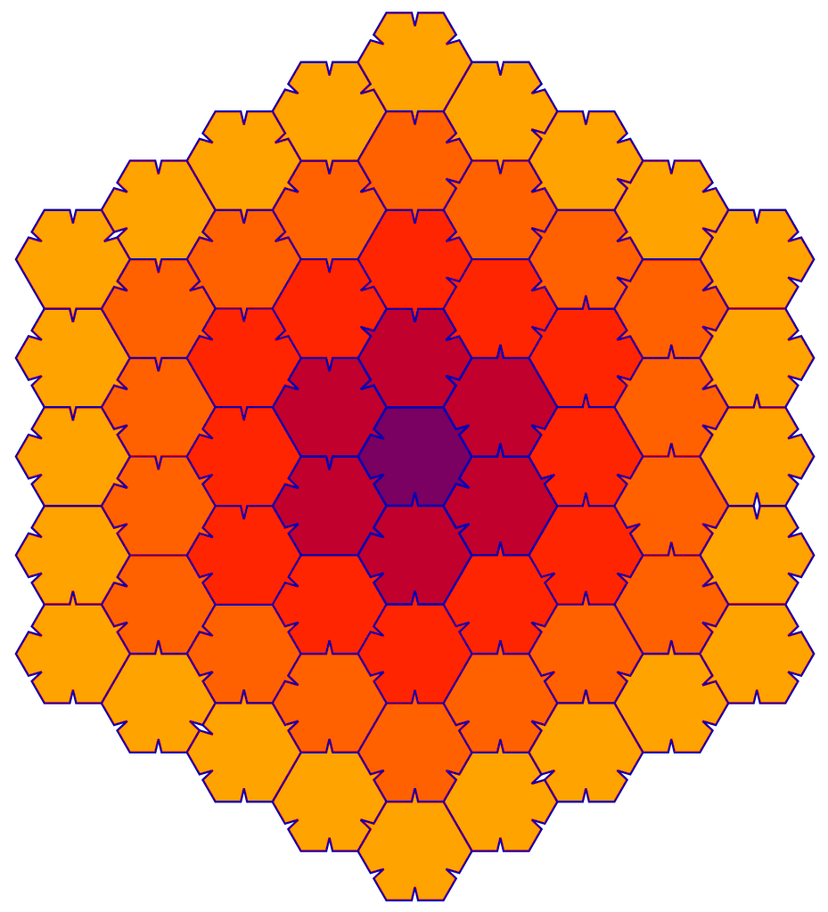 Heesch polygon
A polygon discovered by Robert Amman, formed from a regular hexagon by adding projections on two of its sides and matching indentations on three sides. It may be surrounded by four layers of congruent copies of itself, but not five. See Heesch’s problem.
Source: Wikipedia
Generic parameters
The generic unit declares generic formal parameters, which can be:
- objects (of mode in or in out but never out)
- types
- subprograms
- instances of another, designated, generic unit.
When instantiating the generic, the programmer passes one actual parameter for each formal. Formal values and subprograms can have defaults, so passing an actual for them is optional.
Generic formal objects
Formal parameters of mode in accept any value, constant, or variable of the designated type. The actual is copied into the generic instance, and behaves as a constant inside the generic; this implies that the designated type cannot be limited. It is possible to specify a default value, like this:
generic
   Object : in Natural := 0;
For mode in out, the actual must be a variable. One limitation with generic formal objects is that they are never considered static, even if the actual happens to be static. If the object is a number, it cannot be used to create a new type. It can however be used to create a new derived type, or a subtype:
generic
   Size : in Natural := 0;
package P is
   type T1 is mod Size; -- illegal!
   type T2 is range 1 .. Size; -- illegal!
   type T3 is new Integer range 1 .. Size; -- OK
   subtype T4 is Integer range 1 .. Size; -- OK
end P;
The reason why formal objects are nonstatic is to allow the compiler to emit the object code for the generic only once, and to have all instances share it, passing it the address of their actual object as a parameter. This bit of compiler technology is called shared generics. If formal objects were static, the compiler would have to emit one copy of the object code, with the object embedded in it, for each instance, potentially leading to an explosion in object code size (code bloat).
(Note to C++ programmers: in C++, since formal objects can be static, the compiler cannot implement shared generics in the general case; it would have to examine the entire body of the generic before deciding whether or not to share its object code. In contrast, Ada generics are designed so that the compiler can instantiate a generic without looking at its body.)
Generic formal types
The syntax allows the programmer to specify which type categories are acceptable as actuals. As a rule of thumb: The syntax expresses how the generic sees the type, i.e. it assumes the worst, not how the creator of the instance sees the type.
This is the syntax of RM 12.5
 formal_type_declaration ::=
   type defining_identifier[discriminant_part] is formal_type_definition;

 formal_type_definition ::= formal_private_type_definition
                          | formal_derived_type_definition
                          | formal_discrete_type_definition
                          | formal_signed_integer_type_definition
                          | formal_modular_type_definition
                          | formal_floating_point_definition
                          | formal_ordinary_fixed_point_definition
                          | formal_decimal_fixed_point_definition
                          | formal_array_type_definition
                          | formal_access_type_definiton
                          | formal_interface_type_definition
This is quite complex, so some examples are given below. A type declared with the syntax type T (<>) denotes a type with unknown discriminants. This is the Ada vernacular for indefinite types, i.e. types for which objects cannot be declared without giving an initial expression. An example of such a type is one with a discriminant without default, another example is an unconstrained array type.
In the body we can only use the operations predefined for the type category of the formal parameter. That is, the generic specification is a contract between the generic implementor and the client instantiating the generic unit. This is different to the parametric features of other languages, such as C++.
It is possible to further restrict the set of acceptable actual types like so:
| Generic formal type | Acceptable actual types |
|---|---|
type T (<>) is… |
Definite or indefinite types (loosely speaking: types with or without discriminants, but other forms of indefiniteness exist) |
type T (D : DT) is… |
Types with a discriminant of type DT (it is possible to specify several discriminants, too) |
type T is… |
Definite types (loosely speaking types without a discriminant or with a discriminant with default value) |
Source: Ada Programming
Gaussian Primes
The Gaussian integers are [complex numbers] of the form , where u and v are ordinary [integers] and i is the [square root of negative one]. By defining an analog of the Euclidean algorithm, Gaussian integers can be shown to be uniquely factorizable, by the argument [above]. This unique factorization is helpful in many applications, such as deriving all [Pythagorean triples] or proving [Fermat’s theorem on sums of two squares]. In general, the Euclidean algorithm is convenient in such applications, but not essential; for example, the theorems can often be proven by other arguments.
The Euclidean algorithm developed for two Gaussian integers α and β is nearly the same as that for normal integers, but differs in two respects. As before, the task at each step k is to identify a quotient qk and a remainder rk such that where rk−2 = α, rk−1 = β, and every remainder is strictly smaller than its predecessor, |rk| < |rk−1|. The first difference is that the quotients and remainders are themselves Gaussian integers, and thus are [complex numbers]. The quotients qk are generally found by rounding the real and complex parts of the exact ratio (such as the complex number α/β) to the nearest integers.[^5] The second difference lies in the necessity of defining how one complex remainder can be “smaller” than another. To do this, a [norm function] f(u + vi) = u2 + v2 is defined, which converts every Gaussian integer u + vi into a normal integer. After each step k of the Euclidean algorithm, the norm of the remainder f(rk) is smaller than the norm of the preceding remainder, f(rk−1). Since the norm is a nonnegative integer and decreases with every step, the Euclidean algorithm for Gaussian integers ends in a finite number of steps.